Random Number Generation

1. Inverse Transform Sampling

Suppose that we are able to generate random variables ~ $U[0,1]$. The question is: how to generate other random variables using it?

Note: Random Variable is nothing but a mapping from physical probabilistic event to some predefined set, like mapping of a coin result (face up and face down) to {0, 1}. Now there will be a probability law for occurence of events in physical domain, that translates to probability distribution for our random variable. When we say a random variable X, we are talking about a function in the strictest sense, and when we talk about its probability distribution, we are actually talking about the translated probability law. But for all our purposes, when we say X is sampled from $P_X$, we can just sample from its range (i.e. [0,1] in case of uniform random variable) with law $P_X$, instead of thinking in terms of sampling of events, finding its probablity law and retranslation (you can always reconstrut the event, i.e. calculate inverse). Basically random variables provides a mathematical way to create a standard “pure” probabilistic object and not worry about particularities of physical events, allows for generalizability and wider applicability.

Consider the following operation: We sample x ~ $U[0,1]$, and then we multiply $x$ by $f$ defined by:

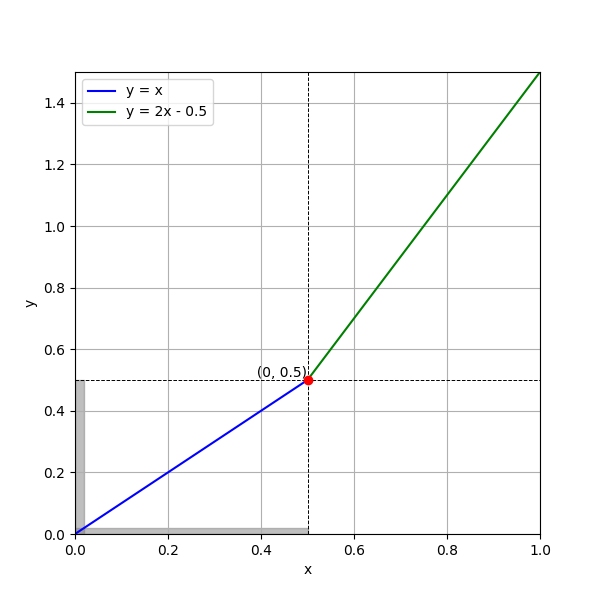
\[\begin{align*} f(x) = \begin{cases} x & 0 \leq x \leq 0.5 \\ 2x - 0.5 & 0.5 < x \leq 1 \end{cases} \end{align*}\]

Now $f([0,1]) = [0, 1.5]$, what is the probability law for this “Derived random variable”? Let us call it $Y$, Surely it is not same as uniform, for $\mathcal{Prob}(Y \in [0, 0.5]) = \mathcal{Prob}(X \in [0, 0.5]) = 0.5$, compared to $\mathcal{Prob}(Y \in [0.5, 1]) = \mathcal{Prob}(X \in [0.5, 0.75]) = 0.25$, and similary $\mathcal{Prob}(Y \in [1, 1.5]) = 0.25$.

Plot of F(x) with shaded region indicating same events

What happened is the shrinking and elongation of events when mapped using a function! Unless the slope is 1, the event size would be different. This gives a natural way to create arbitary distribution, suppose $F: [0, 1] \to [-\infty, \infty]$ be a continuous, monotonic (else we have consider to different segments) and differentiable function (can be non-differentiable at finitely many point though). Let $Y$ be a derived r.v, defined by $F(X)$ (which just means sample of $Y$ = image of sample of $X$ under $F$).

\[\begin{align*} \mathcal{Prob} \left(Y \in [y, y + \delta y] \right) &= \mathcal{Prob} \left( F(X) \in [y, y + \delta y] \right) \\ &= \mathcal{Prob} (X \in [F^{-1}(y), F^{-1}(y + \delta y)]) \\ \end{align*}\]

Here as the $X$ is uniform, only the size of interval matter, assuming straight line with slope $F^\prime(F^{-1}(y))$, and $\delta y$ = $F^\prime \delta x$:

\[\begin{align*} \mathcal{Prob} \left(Y \in [y, y + \delta y] \right) &= \mathcal{Prob}(X \in [0,\delta x]) \\ P_Y(y) \delta y &= 1 \cdot \delta x \\ &= \frac{\delta y}{F^\prime (F^{-1}(y))} \\ \end{align*}\]

Hence, $P_Y(y) = 1/F^\prime (F^{-1}(y))$. Okay, we found out that - Distribution of derived r.v is not uniform and computed what exactly it is. But, how to do “converse”, as in, is it always possible to find certain function $F$ s.t we get any desired probabilty distribution? Yes! For the $F$ is rather a very special and unique¹ to every distribution! Let us ponder over this F, and try to make intutive sense in relation to the distribution. For starters, what is the CDF of F?

CDF (cummulative distribution function) is nothing but a function over range of r.v, s.t CDF(x) = Probability of $X \leq x$.

\[\begin{align*} \mathcal{CDF}(y) &= \mathcal{Prob}(Y \leq y) \\ &= \int_{-\infty}^y P_Y(y) \delta y \\ &= \int_{-\infty}^y 1/F^\prime(F^{-1}(y)) \delta y \\ \end{align*}\]

Let $G = F^{-1}$, this implies $G^\prime(y) = 1/F^\prime (x)$², where $y = F(x)$. Doing this substitution above we get

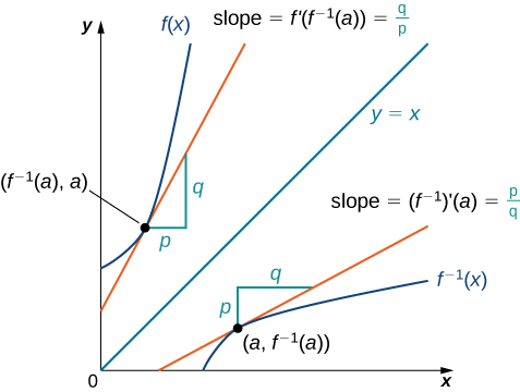
Inverse Function. Source: https://courses.lumenlearning.com/suny-openstax-calculus1/chapter/derivatives-of-inverse-functions/

\[\begin{align*} \mathcal{CDF}(y) &= \int_{-\infty}^y G^\prime(y) \delta y \\ &= G(y) \end{align*}\]

We assumed $F(+-\infty) = 0$ (consequently the inverse is 0) as otherwise distribution will be illdefined (i.e. total probability = 1 be under pressure). I.e. the CDF is nothing but the inverse of $F$. So we have found a way to generate any random variable:

1. Find the CDF
2. Compute its Inverse
3. Using it find the derived r.v with $U[0, 1]$, it will generate the required r.v!

There is a much cleaner (natural, to be precise) way to arrive at this conclusion. The CDF ($G$) is continuous, sufficiently differentiable and monotonic. Its is a function from domain of r.v. to [0,1]. This provides a very natural translation (map) between 0 to 1 strip and our domain. Here $P_Y(y) = G^\prime(y)$ (DIY, start with identifying the equivalent region / event), and this is the desired PDF (probability density function, or $P_Y(y)$, for pdf is nothing but derivative of CDF)!

2. How to generate Uniform [0,1]

This is a very broad topics in its own rights, and I am not the merrier myself. There are several lines of enquiry -

1. Can there exist any true random event in nature? If yes, we would leverage it (we do, for it might not be random but is sufficiently so, leverage atmospheric noises and other stochastic processes for random number generation. Refer here). This is a deep philosophical question, for if there is no true randomness, for there might not be free will. And as such, we defer this dialogue to the reader itself.

2. A computer program (equivalent to a deterministic turing machine) can’t create a random number, for it is by nature deterministic, and any output of the algorithm³ can be traced back to the initial “generator” (as otherwise, without any change in initial input, the output always remains the same). But that doesn’t mean algorithmic “random” generation is useless, in many places we just want number that appear to be random, i.e. in theory they all are related by some intricate pattern (namely the algorithm), and we want that the decipher, given the algorithm remains a mystery, shouldn’t be able to solve it in a short time. This field is called pseudo random generation. We state one such algorithms and defer any discussions on merits and quantification of these algorithms, for it requires a through analysis on what makes a good generator (preceded by a general theory of generators).

2.1 Von Neumann Algorithm

Before we detail the algorithms, there is a little problem: Computers can’t work with real number, it has finitely many bits and as such can only store integers. So what we are going to do is, generate numbers (rational, and ideally uniformly) of form $m/M$, where $M$ is fixed to some large number and $m \sim [0, M-1]$. The algorithm is very simple, let us see with an example. Pick $M = 10000$, so $m \in [0, 9999]$.

1. Pick any initial $m$ (seed). One can also pick this seed using “physical” randomness like coin flip or noise.

2. Square the number, remove the first 2 digits (most significant digits, left side) and keep the new first 4 digits. I.e. out of the 8 digits (square of 4 digit number can at max have 8 digits, think from the multiplication table thing we do or any other way …), keep the middle 4. In other words, we define recursion as follows $m_{i+1} = [m_i / 100] \text{ mod } 10000$, where “[]” is the integer part (removes decimal, or equivalent to removing last 2 digits).

Example, $m_0 = 5232 \to m_1 = 3738 \to m_2 = 9726 \to m_3 = 5950 \cdots$, and the random output being 0.5232, 0.3738, and so on.

class VonNeumannAlgorithm():
    def __init__(self, m0=5232):
        self.current_m = m0
        self.sequence_m = [m0]
    def generate_next(self):
        self.current_m = int(self.current_m**2 / 100) % 10000
        self.sequence_m.append(self.current_m)
        return self.current_m

generator = VonNeumannAlgorithm()
print(f"m0 is: {generator.current_m}")

for i in range(1,100):
    generator.generate_next()
    print(f"m{i} is: {generator.current_m}")

Now there are a few questions, first why (and how) does it mimic uniform distribution. And secondly, is it any good. For later, all we can do, informly, is perform some checks. For instance, aggregate results of distribution like $n^\text{th}$ moments (expectation of $m^n$) or correlation between $m_i$ and $m_j$. I.e. calculate computationally and compare it to analytical results. Also one must not forget, at max we can generate a series of 10000 numbers, as after that we are bound to cycle back again. And that the series will remain the same, i.e. say $L$ be the cycle length, then $m_{L+i} = m_i$ and thus is not random anymore. For the former, there are no (not to my little knowledge) any concrete results on similarity with uniform distribution. It is ofcourse, not completely uniform distribution, breaks as number of points reach close to cycle length, also the distribution is concentrated in some regions. But the idea is, when we square the middle portion (those 4 digits), they show the most randomness as they are influenced by the entire string, compared to the trailing digits, and as such can take any value. This is the best I have.

3. References

1. Paper on various pseudo random generation algorithms

2. Paper on properties of good pseudo random generator

3. Hardware Random Number Generator

4. Pseudorandom Number Generator

4. Notes

1. Unique, in so far as to say CDF is unique. For random variable can be different, and yet there CDF be same. The reason, though probability is same for that region, but who said the converse mapping need be the same? Consider 2 r.v X and Y. And physical event be picking a number between 0 and 1 (uniformly). X is simply that number and Y is 1 - that number. Suppose the physical events came 0.4, X takes the value of 0.4, whereas Y takes value of 0.6. Now if you try to computer $P_X(x)$, it is nothing but $U[0,1]$, and also $P_Y(y)$ is nothing but $U[0, 1]$! (think, Y is just X, only that each number is off by 1. Do your calculuations in X and shift the result by 1) ↩︎

2. Quite simple to see. First one must understand, inverse is nothing but the same function (visualize geometrically on cartesian plane) ,taken mirror image about $y = x$. See the attached image above. Now understand that the slope is same as measured from the axis, for it is the same function looked that way! In other words, let a vector in the direction of tangent to F be (a,b) , now when you rotate the function the derivative is also rotated in the same way (imagine F as sum of piecewise linear function, tangent is nothing but the function itself in this case). When you rotate a (a, b) vector around $y = x$, the new vector is (b, a), for component along x becomes component along y and component along y becomes component along x. The slope given by b/a becomes a/b which is but inverse. ↩︎

3. Church-Turing hypothesis states that turing maching and $\lambda$ calculus (~premitive form of programmign language) are equivalent in terms of generating algorithms. ↩︎