Pursuit Problem

Problem-1 Statement

Consider a simple setup, an individual is stationed at each of the vertex of a N-sided regular polygon. From t = 0, they are always moving towards the next person. When will they all meet, and what is the path followed by any one of them?

Solution-1

Before we begin, we must realize one simple idea - Radial and perpendicular velocity. Consider 2 particles A and B, A be at rest and B be moving at velocity \(v_x\) and \(v_y\) (as shown below).

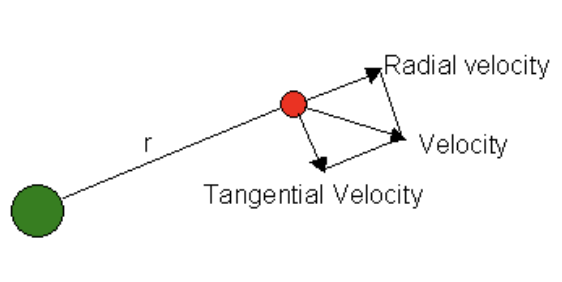
Here \(v_x\) is always radial to the line AB and \(v_y\) is always tangential to the line AB. The distance between A and B is only affected by \(v_x\) and not \(v_y\)! On surface one might say \(v_y\) does alter the distance, using some notion of pythagorian equality, but one should note \(v_y\) is “always” perpendicular to the line AB. Its like the velocity of a ball being hurled in a circle, it would have added distance if it kept moving (even if for a moment) but rather it is always changing just like in a circle.

Let us consider the case of an equilateral triangle ABC. Let us first find the time of collision (by symmetry which will occur at the very center, a point symmetric w.r.t all). A is moving towards B with velocity \(v\) and B is moving towards C with the same velocity. Let us see the situation from reference frame of A, B is effectively moving towards A with a velocity \(v + v \cos (\pi/3)\), which is \(3v/2\). This is but for that very instant. But owing to symmetry, one can easily see the triangle ABC after a \(\Delta t\) interval is also an equilateral triangle¹, thus this is always the radial velocity. So the time of collision would be \(s / (3v/2)\) \(= 2s/3v\). For a general N-sided regular polygon, it would be \(s / v[1+\cos((N-2)\pi/N)]\), where \(s\) is the side length. As a special case, let us see what happens at N = \(\infty\), i.e. a circle. The time becomes infinite! Which makes sense, as the pursuer and the chased point are always at \(\pi\) angle w.r.t to each other, there motion is just rotation in the circle.

The path followed is quite intutive to visualize, for the regular 4-gon following is the trajectory.

Pursuit Problem trajectory on a Square. Ref: https://en.wikipedia.org/wiki/Pursuit_curve

Problem-2 Statement

Let us a consider a 2 player pursuit problem where we can derive the equation for the curve easily. Let A and B be 2 points on the plane. A starts moving along a straight line (\(x=0\)) at a constant velocity \(v_A\) (A never deviates from the first chosen direction). B is the pursuer, starting at (\(x_0, y_0\)), and is constantly changing the direction as to follow A, with velocity \(v_B\). What is the time of collision, where does the collision takes place and what is description of path traced by B.

Solution-2

Following image shows visually our situation (replace P with B). B is always moving towards A and A is moving nonchalantly along a straight line.

A simple pursuit curve in which P is the pursuer and A is the pursuee. Ref: https://en.wikipedia.org/wiki/Pursuit_curve

This is a very routine problem, just write the time derivates of \(x\) and \(y\), and pray it is solvable in whatever capacity². The 2 time derivatives are -

\[\begin{align*} \dot{x} &= \frac{-v_b x}{\sqrt{x^2 + (y - v_a t)^2}} \\ \dot{y} &= \frac{-v_b (y - v_a t)}{\sqrt{x^2 + (y - v_a t)^2}} \\ \end{align*}\]

Where \(v_a\) and \(v_b\) are velocities of A and B. Above is the standard \(v_b \cos{\theta}\) and \(v_b \sin{\theta}\) (with sin and cosine expanded in terms of \(x\) and \(y\)). Or one can also directly see it as \(\vec{v_b} = v_b \widehat{AB}\). This problem posits certain symmetry, allowing us to do a switch of variables and rendering it only a function of variables on lhs. To wit, \(w(t) = y(t) - v_at\), where \(\dot{w} = \dot{y} - v_a\). We therefore get 2 non-linear differential equations. As the task of solving \(x(t), w(t)\) at the moment seems hard, we first attempt finding \(w(x)\).

\[\begin{align*} \frac{dw}{dx} &= \frac{\frac{dw}{dt}}{\frac{dx}{dt}} \\ &= \frac{v_bw + v_a \sqrt{x^2 + w^2}}{v_bx} \\ &= \frac{w}{x} + \frac{v_a}{v_b}\sqrt{1 + \frac{w^2}{x^2}} \\ \end{align*}\]

Let us call \(v_a/v_b = \eta\) and as this is a standard homogeneous equation, we do the natural substitution \(w(t) = u(t)x(t)\). Here \(\frac{dw}{dx} = \frac{du}{dx}x + u\), and using it in our main equation we get

\[\begin{align*} \frac{du}{dx}x &= \eta \sqrt{1 + u^2} \\ \int \frac{du}{\sqrt{1 + u^2}} &= \int \eta \frac{dx}{x} \\ \sinh^{-1}(u) &= \eta \ln(\vert x \vert) + C_1 \\ \end{align*}\]

In the last step, we note the integral of \(1/\sqrt{1+u^2}\) is nothing but \(\ln{\vert u + \sqrt{1+u^2} \vert}\) (replace \(u\) by \(\tan{\theta}\) and noting that the \(\int \sec{\theta}d\theta = \ln\vert \sec\theta + \tan\theta \vert\)). Also \(\sinh(x) = (e^x - e^{-x}) / 2\), finding \(x\) in terms of \(\sinh(x)\) easily yields our claim³. Finally we have \(u(x) = \sinh(\ln(\vert x \vert^\eta C_1^\prime))\), \(C_1 = \ln(C_1^\prime)\), on expanding we get \(\frac{1}{2}\left[\vert x \vert^\eta C_1^\prime - \frac{1}{\vert x \vert^\eta C_1^\prime}\right]\).

Now we have got \(u(x)\), consequently we have \(w(x) = ux\). We finally have \(\dot{x}\) in terms of \(x\) and can look forward to solving it. To simplify algebra, note that if you take \(x\) common in denominator you get \(\sqrt{1+u^2}\) below. \(u\) is \(\sinh\) something. We know \(\cosh(x)^2 - \sinh(x)^2 = 1\), so we get the equation with \(\text{sech}\) something in numerator. You don’t need this identity, just go ahead and put the value of \(u\) here and solve (trying to save just one extra line). Doing all this we get, \(\dot{x} = -2v_b / \left[\vert x \vert^\eta C_1^\prime + \frac{1}{\vert x \vert^\eta C_1^\prime}\right]\). This is a elementary integral, solving which we get the implicit equation -

\[\begin{align*} -2v_bt &= \left[\frac{\vert x \vert^{\eta+1} C_1^\prime}{\eta + 1} - \frac{1}{(\eta-1)\vert x \vert^{\eta-1} C_1^\prime}\right] + C_2 \\ \end{align*}\]

Though this is implicit from \(x(t)\), it explicit in terms of \(t(x)\). This allows us to express \(y(x) = w(x) + v_at\). Let us simplify the express a bit before calling it a day.

\[\begin{align*} y(x) &= u(x)x - \frac{v_a}{2v_b} \left[\frac{\vert x \vert^{\eta+1} C_1^\prime}{\eta + 1} - \frac{1}{(\eta-1)\vert x \vert^{\eta-1} C_1^\prime} + C_2 \right] \\ &= \frac{1}{2}\left[\vert x \vert^{\eta+1} C_1^\prime - \frac{1}{\vert x \vert^{\eta-1} C_1^\prime}\right] - \frac{v_a}{2v_b} \left[\frac{\vert x \vert^{\eta+1} C_1^\prime}{\eta + 1} - \frac{1}{(\eta-1)\vert x \vert^{\eta-1} C_1^\prime} + C_2 \right] \\ \end{align*}\]

You can plug the initial values for \(C_1, C_2\) at the appropriate places to find its value. One last thing, this equation in not valid for \(\eta = 1\), as our integral equation for \(x\) would have yeilded \(\ln\vert x \vert\) instead of a power of \(x\). For \(\eta = 1\), the implicit equation for \(x(t)\) would be, \(-2v_bt = \frac{\vert x \vert^2 C_1^\prime}{2} + \frac{\ln\vert x \vert}{C_1^\prime} + C_2\). Here the \(y(x)\) would be

\[\begin{align*} y(x) &= u(x)x - \frac{v_a}{2v_b} \left[\frac{\vert x \vert^2 C_1^\prime}{2} + \frac{\ln\vert x \vert}{C_1^\prime} + C_2 \right] \\ &= \frac{1}{2}\left[\vert x \vert^{2} C_1^\prime - \frac{1}{C_1^\prime}\right] - \frac{1}{2}\left[\frac{\vert x \vert^2 C_1^\prime}{2} + \frac{\ln\vert x \vert}{C_1^\prime} + C_2 \right] \\ &= \frac{1}{2}\left[ \frac{\vert x \vert^{2} C_1^\prime}{2} - \frac{\ln\vert x \vert}{C_1^\prime} - \frac{1}{C_1^\prime} - C_2 \right] \end{align*}\]

Here \(C_1 = \sinh^{-1}\left(\frac{y_0}{x_0}\right) - \ln\vert x_0 \vert\) and \(C_2 = - \left[ \frac{\vert x_0 \vert^2 C_1^\prime}{2} + \frac{\ln\vert x_0 \vert}{C_1^\prime}\right]\).

Following is the python code to generate trajectory for \(\eta = 1\) case -

import numpy as np
import matplotlib.pyplot as plt

# Input parameters
x0 = 2.0  # Example: starting x-coordinate
y0 = 0.0  # Example: starting y-coordinate

# Define constants
C1 = np.arcsinh(y0 / x0) - np.log(np.abs(x0))
C1_prime = np.exp(C1)
C2 = -((np.abs(x0)**2 * C1_prime) / 2 + np.log(np.abs(x0)) / C1_prime)

# Define the function f(x)
def f(x):
    return 0.5 * ((x**2 * C1_prime) / 2 - np.log(x) / C1_prime - 1 / C1_prime - C2)

# Generate x values to the left of x0, but still positive
x_vals = np.linspace(1e-6, x0, 1000)
y_vals = f(x_vals)

# Mask to ensure we only plot values where f(x) > 0 (first quadrant)
mask = y_vals > 0
x_vals = x_vals[mask]
y_vals = y_vals[mask]

# Plotting
plt.figure(figsize=(8, 5))
plt.plot(x_vals, y_vals, label='f(x)', color='blue')
plt.scatter([x0], [y0], color='red', zorder=5, label=f'Start ({x0}, {y0})')
plt.title("Pursuit Curve")
plt.xlabel("x")
plt.ylabel("f(x)")
plt.xlim(left=0)
plt.ylim(bottom=0)
plt.grid(True)
plt.legend()

# Add padding on both axes
x_pad_max = 0.3 * (x_vals.max() - x_vals.min())
y_pad_max = 0.3 * (y_vals.max() - y_vals.min())
x_pad_min = 0.1 * (x_vals.max() - x_vals.min())
y_pad_min = 0.1 * (y_vals.max() - y_vals.min())
plt.xlim(x_vals.min() - x_pad_min, x_vals.max() + x_pad_max)
plt.ylim(y_vals.min() - y_pad_min, y_vals.max() + y_pad_max)

plt.show()

For \((x_0, y_0) = (2, 1)\) the plot is as follows -

Pursuit trajectory for 2 body problem with eta = 1

Before signing off,

1. If \(\eta > 1\) i.e. \(v_a \gt v_b\) no collision takes place (Intutive as well as in our explicit \(t(x)\) equation, for \(x \rightarrow 0\) we have \(t \rightarrow \infty\)).

2. If \(\eta < 1\) i.e. \(v_a \lt v_b\) collision takes place on \(t = -\frac{C_2}{2v_b}\) at \(y = -\frac{\eta C_2}{2}\).

3. If \(\eta = 1\) i.e. \(v_a = v_b\) no collision takes place (In our explicit \(t(x)\) equation with \(\eta = 1\) , for \(x \rightarrow 0\) we have \(t \rightarrow \infty\)). Unlike first case, this time because log grows slowly around 1 (by \(1/x\)) compared to other inverse powers of \(x\), the pursuer gets quite close and starts tailing instead of being left behind. A better view is from looking at \(w\), which is the measure of vertical separation between them at any given time. Around \(x = 0\), for \(\eta = 1\) it is constant (\(-1/2C_1^\prime\)) whereas for first case it grows to infinity.

Notes

1. What else could it be? All angles and sidelengths have to be the same because of symmetry in there motion. ↩︎

2. Solvable in the highest order refers to finding \(x(t)\), \(y(t)\), \(y(x)\) explicitly. Here we will get implicit equation of \(x\) and \(t\), and explicity equation of \(y(x)\). ↩︎

3. Let \(\sinh(x) = y\) and \(e^x = t\), we have \(y = (t - 1/t)/2\). Converting into quadratic equation, \(t^2 - 2yt - 1 = 0\), we find the solution \(t = y \pm \sqrt{y^2 + 1}\). As \(t\) is always positive, we can discard the negative solution, and consequently we have \(x = \sinh^{-1}(y) = \ln(y + \sqrt{y^2 + 1})\). ↩︎